
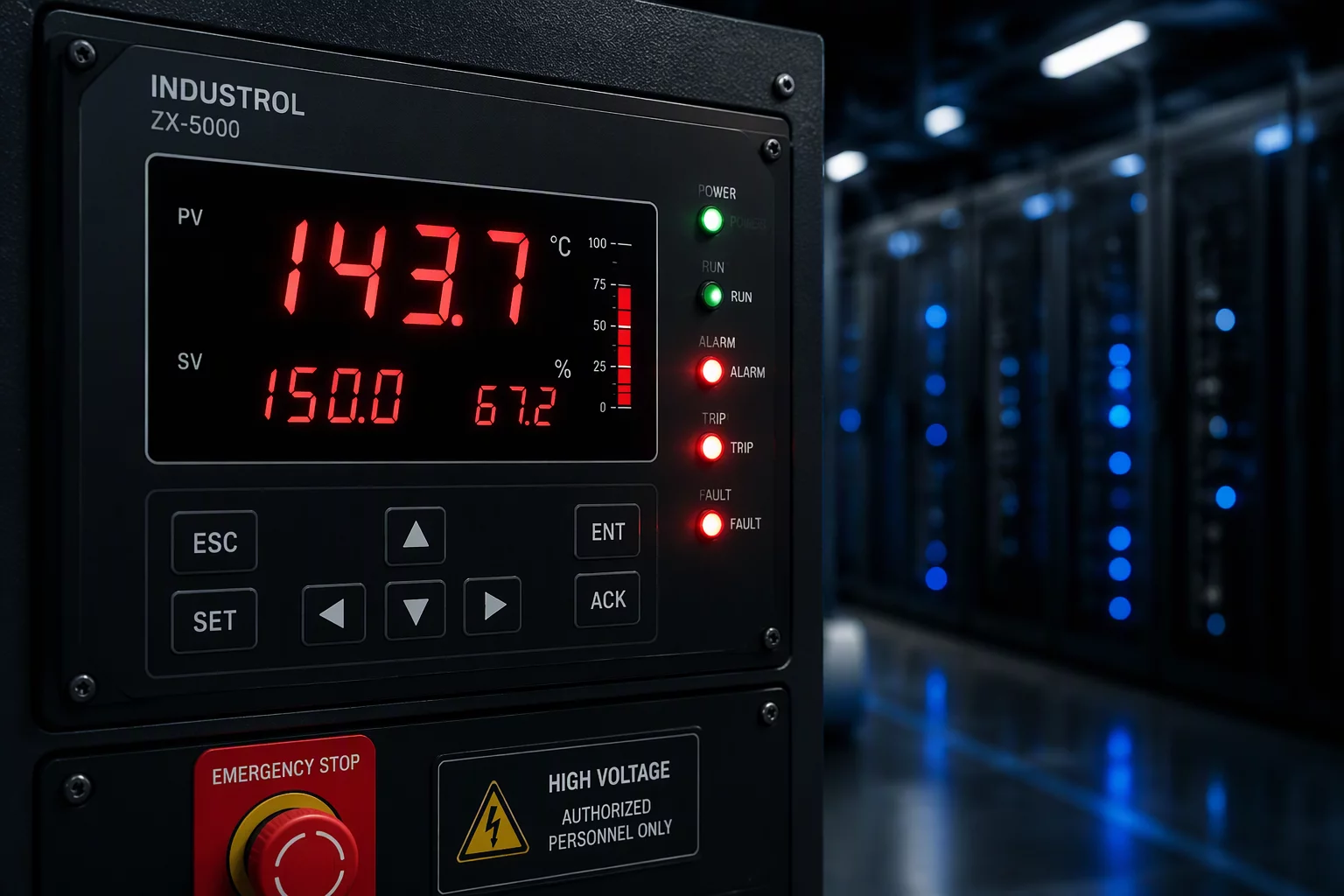
The Illusion of Static Ambient and Auxiliary Conditions
Uncontrolled background parameters represent the most insidious failure mode in classical factorial setups. An experimenter constructs a 2³ full factorial design, records target settings into execution sheets, and assumes peripheral systems maintain uniform outputs. In real operational settings, pumps degrade gradually, ambient relative humidity creeps upward as afternoon shifts begin, and electrical resistance shifts under continuous load. Because no team member records telemetry for these auxiliary baselines, the mathematical model treats their quiet fluctuations as pure unexplained experimental error, or worse, assigns their consequences to an innocent primary factor.
Consider an injection molding trial evaluating resin temperature, injection speed, and pack time. The chiller supply line remains set to 18°C on the analog dial. During morning runs, cooling water circulates at exactly 18.2°C. By run twelve, heat absorption from neighboring production lines drives chiller water inside the test press manifold up to 24.6°C. Because the design matrix assigns high pack times predominantly to later afternoon batches due to poor run-order randomization, part shrinkage decreases noticeably. The regression software promptly credits pack time with a massive, statistically significant stabilizing effect. In reality, the creeping chiller loop temperature caused every millimeter of that dimension variance.
-
01
Continuous Sensor Validation Install automated data loggers directly at point-of-use tooling rather than relying on remote wall thermostats or manual machine dial setpoints.
-
02
Run Order Randomization Defense Strict randomized trial execution distributes time-dependent drift evenly across treatment combinations, preventing false main effect confounding.
-
03
Residual Trend Diagnostics Inspect residual vs. run order scatter plots immediately; persistent slope patterns highlight hidden non-constant settings operating behind the scenes.
Converting Silent Hazards into Explicit Experimental Blocks
Detecting variable instability during pilot execution demands a shift from passive trust to systematic constraint audits. Before freezing a testing schedule, catalog every environmental, auxiliary, and raw material stream feeding into your equipment. When an auxiliary setting cannot maintain hard physical tolerances, redesign the test structure around that instability. Group runs into balanced blocks corresponding to operational shifts, chemical supply batches, or thermal cycles. Alternatively, register the fluctuating measurement as an explicit continuous covariate inside your analysis of covariance (ANCOVA) model, adjusting response means mathematically.
“A machine parameter is never a constant simply because your engineering protocol omitted its sensor from the data collection sheet.”
Post-trial verification relies heavily on diagnostic charting. Plotting model residuals against chronological execution sequence exposes non-constant behavior immediately. A random scatter confirms that background noise remained stationary throughout testing. A curved or diagonal drift across residuals reveals that an unaccounted variable silently moved the baseline. Catching this pattern early saves engineering teams from authorizing expensive tooling modifications based on false interaction models.
Add Engineering Note
Share your observations or validate experimental factor assumptions.